ID4CS Prototype 2 Tutorial

Description

Here you will find how to get, run and experiment with the second prototype of the ID4CS optimization system.

For details on the different types of models and how to load them, see ID4CS Model Types.

For details on specific characteristics used by the elements, see ID4CS Characteristics.

Run Prototype 2

Simply execute the ID4CS.bat file :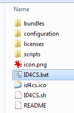

This is what you will see on the first run : ID4CS first run

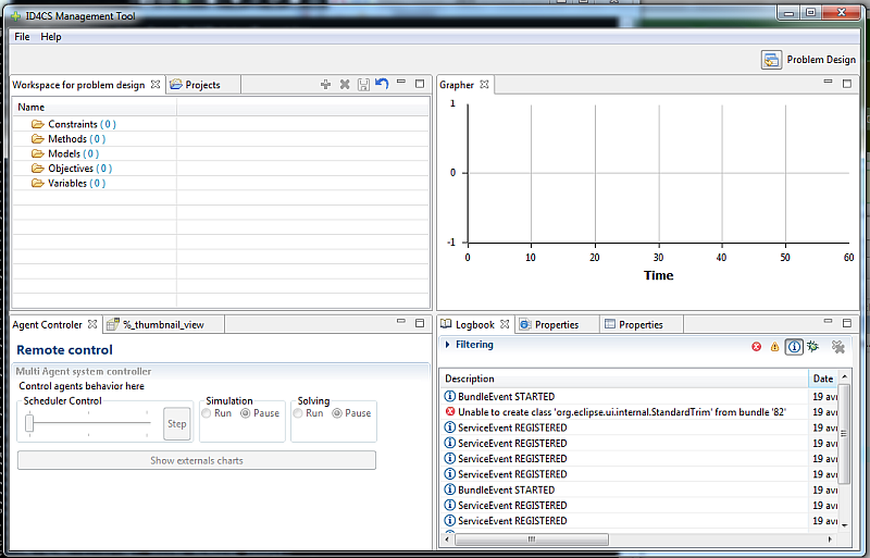
Description of the ID4CS tool

Upper left window

The workspace for problem design. It contains the variables, models, methods, constraints, objectives, etc. for defining a problem. It also contains, in the second tab, the different projects and problems that have been created in the workspace.

Upper right window

The "Grapher" tab shows the evolution of all the variables of a problem during its execution. The following tabs appear when opening problems and show the graph of the problem (link between the variables, models, etc.).

Lower right window

Shows and enables editing of the properties of the different elements in the workspace.

Lower left window

Control of the execution of the problem currently open in the upper right window. The second tab shows an overview of the current problem.

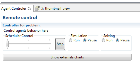
The "show external charts" button launches another windows which shows the evolution of the value of each variable of a problem, along with its associated criticality;

Preferences

The menu "Preferences" gives the possibility to specify the Scilab executable to use.
For now Scilab works on Windows with Scilab 5.3.3 and on Linux with Scilab 5.4.1 minimum.

Create a first problem

As a first tutorial, we will create a mini "problem" with a simple model m with two inputs i1 and i2, and one output o, calculating m(i1,i2)= i1+i2.

1. Launch proto2

2. In the "workspace" (a tab in the upper left window), right-click on "Models" and choose "Create resource". Name it m for instance, check C++ type, click "Next" and click on "Open DLL file". The dll file will be responsible for the actual calculus of the model. Get a zip file that contains SUMF64.dll, a simple model calculating the sum of its two inputs.

3. In the same workspace, create variables i1, i2 and o (right click on the "variables" folder).

4. The workspace can be saved using the "floppy" icon.

5. Open the "Projects" tabs.

6. Right-click on an empty space an choose "Create new project". Name it "Tutorial1" for instance.

7. Right-click on the "Problems" folder under your new project and choose "Create new problem". Name it "Problem1" for instance.

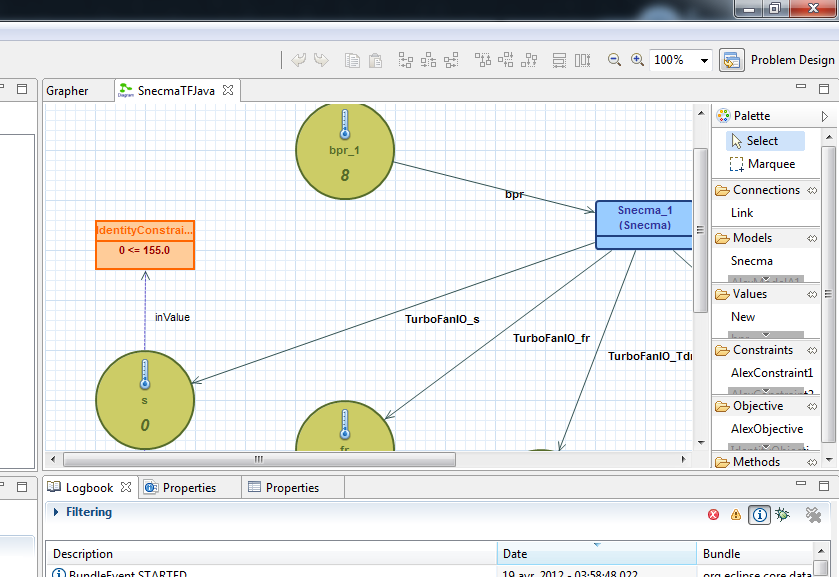
8.Creating a new problem will open a new tab in the upper right with a "blueprint" background on which we will "draw" the problem by graphically adding the elements from the problem. On the right of this tab, there is a "Palette" containing the element created previously : m, i1, i2, o. Click on an element and click on the blueprint to add the element to the problem.

9. Drag-and-drop the elements onto the blueprint, then choose the "link" element to link these element together : i1 and i2 as inputs of m and o as output.

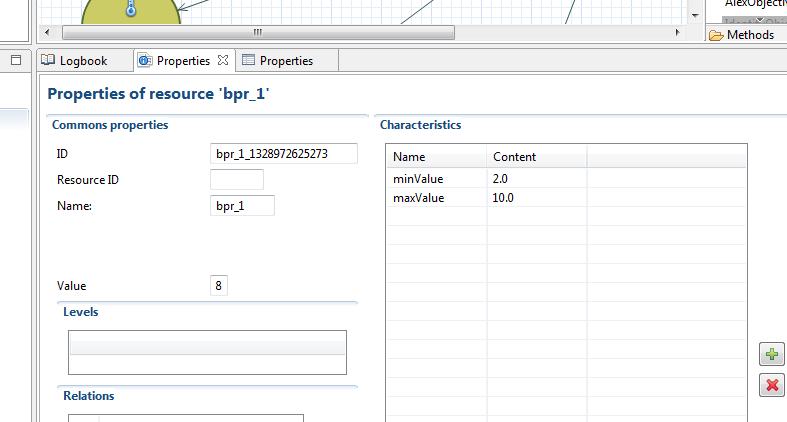
10. Click on the "Properties" tab (lower right window) and then on variable i1. Put a chosen value in the "value" field. Do the same with i2.

11. The graph can be saved by pressing ctrl+S and enter.

12. We are now ready to "run" the problem. For this, we will use the "Controller" (in the lower left). Ensure that only "simulation" is checked and click on the "Step" button several times (as the first steps enable the agents to initialize). You can see that the value of o is updated both on the visual representation of the problem, and on its properties tab. If you change an input value, the agents will re-calculate and propagate the values through the problem.

Adding constraints, objectives and solving the problem

1. In the workspace tab, create a new constraint C1 based on the "identity" java model (this means that the constraint will simply take the value of a variable. We will later be able to work on a function of the variable, for instance the square root, etc.).

2. In the properties tab, add an "input" : click on the green "+" button in the "inputs" section. Change its name to "inValue" and its type to FLOAT_64. Do the same for an output (name it "output" and choose FLOAT_64 for its value).

3. Add the C1 constraint to the problem (click on C1 in the palette and the on the blueprint, next to i2).

4. In the property tab of the constraint you just added, choose "operation : >=" and "Threshold : 12".

5. Add a link between i2 and C1.

6. In the workspace tab, create a new objective O1 based on the identity java model.

7. In the properties tab, add an "input" : click on the green "+" button in the "inputs" section. Change its name to "inValue" and its type to FLOAT_64. Do the same for an output (name it "output" and choose FLOAT_64 for its value).

8. Add the O1 objective to the problem next to o.

9. In the properties tab of O1, check that "Optimisation" is set to "Minimize".

10. Add a link between o and O1.

11. Make sure that "solving" is checked in the "Controler", click on "show external charts", choose a speed with the slider and look at the charts as the agents solve the problem.

12. You can add a constraint to the other variable to see the system converge. Feel free to modify this problem and see how the system reacts.

Alexandrov problem

We will now load and solve the Alexandrov problem.

1. Make sure ID4CS is closed.

2. In the ID4CS folder (where you executed the ID4CS.bat file to run proto1), there is a "workspace" folder containing the resources, the projects and the problems. The current workspace only contains what we created in tutorial 1. Rename it to "workspaceTUTO1".

3. Copy the Alexandrov workspace there. Make sure the folder is simply called "workspace" and directly contains a "ressourceLib" folder.

4. Run proto1. As you can see, the "Workspace" tab now contains all the resources of the Alexandrov problem : c1, c2, s, l1, l2, m1, m2, a1, a2, o1.

5. In the "Projects" tab, open the "alexandrov" problem. You can now see it represented graphically on the right.

6. Click on the "Show external charts" button

7. In the "Controller", make sure the "simulation" and "solving" are checked and choose a solving speed on the "scheduler control" slider.

8. In the external charts you can see how the problem is solved.

NOTE : if you minimize the console window (terminal), the prototype runs faster.

Snecma Test Case 1

As in the previous step, we will be loading and running an already designed problem: the Snecam Test Case 1.

1. Ensure that ID4CS is closed.

2. Rename the "workspace" folder to "workspaceALEX" (if you previously did the Alexandrov tutorial).

3. Copy the Snecma Test Case 1 workspace there. Make sure the folder is simply called "workspace" and directly contains a "ressourceLib" folder.

4. Run ID4CS, explore the problem and make the system solve it. You can see that the system stabilises on values of the pareto front as seen in the Snecma Test Case 1 document (cf. ID4CS web site, Deliverable D12).